Generative AI in the latent space
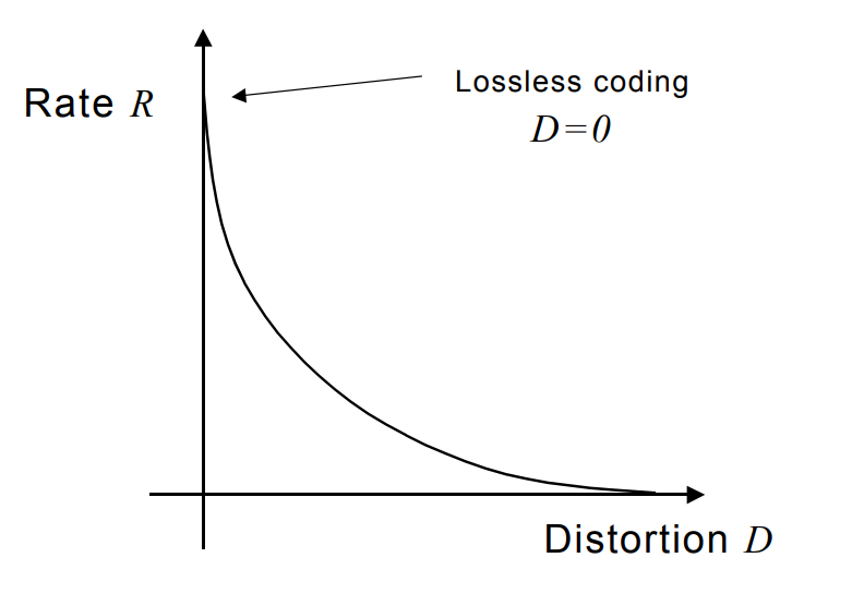
Real world perceptual data (images, language, audio, 3D shapes) has a large amount of redundancy. In other words, the number of bits needed to perfectly represent a sample in one of these data modalities is very high, but a large percentage of those bits are actually spent in representing very fine, minute details. If we were to find a way to compress the information needed to represent an data sample in one of these modalities, then relatively few bits would suffice to capture the high level perceptual detail. For example, high-fidelity audio is about 9 Mbps but MP3 audio is only about 200-300 kbps and telephone voice is just 64 kbps. The drop in telephonic voice audio quality is obvious. This tradeoff between the number of bits used to represent data, and the distortion (which is loss in information, and in a practical system it is typically the reconstruction error) is formally captured in classical information theory using a rate-distortion curve. This is typically a convex curve with rate on the Y axis and distortion on the X axis:
Self-supervised learning methods learn a network that compress information, subject to a specified distortion criterion (e.g. L2 reconstruction error). In doing so, they provide a compressed representation of each data sample. For example an image which is typically represented as a tensor of size (C=3, H, W) might compress to say \((C=4, h<<H, w<<W)\). This compressed version is much more computationally amenable to diffusion modeling. This is the main message of [0]. Denoising Diffusion Probabilistic Models are very sensitive the the size of the object they are generating, because unlike a simple supervised learning problem where the output of the network is a collection of C logits (for C classes, in a classification problem) or a single real number (for a regression problem), the output of a denoising network is the predicted noise tensor, which is of the same size as the original data object or the noised data object (i,e, (C, H, W) in the case of an image). Therefore doing diffusion modeling in the original data space requires spending a lot of compute to capture very fine, imperceptible details in the object. Instead, it is possible to:
- First do representation learning on the data, to compress it. Say, using an autoencoder.
- Then do diffusion model, just as before, but on the compressed representation of the data.
- At sampling time, the learnt diffusion model will produce samples in the latent (compressed) space. These generated samples then need to be passed through the decoder portion of the auto-encoder, to produce samples in the original (non latent) data space.
Stable diffusion, and I think pretty much all image-generation (and possibly all competetive video generation) models of today use this 2-step structure. In practice, we can do a bit better. The problem with the above approach is that the final generated samples in the original data space are lossy, i.e. since they are the output of the decoder portion of a compression model, they necessarily cannot capture high-resolution perceptual details that are present in the original uncompressed data samples. To address this shortcoming, the following approach is proposed in [0]:
- Train a Variational Auto Encoder, but with a modification: the loss isn’t just L2 reconstruction loss but also perceptual loss (using VGG features) and an adversarial loss computed using an additiona discriminator attached to the decoded images.
- The latent \(z\) is compressed, i.e. it looses high frequency detail. The decoder alone produced blurry images lacking high frequency details. The discriminator forces reconstructions to lie on the natural image manifold, and as a result the overall decoder learns to “hallucinate” realistic fine details, which cannot be recovered from the latent \(z\) alone.
- The diffusion model portion remains unchanged.
The overall effect of this is to generate data samples via diffusion modeling, containing high level (low frequency) details but lacking very fine (high frequency) details, and then relying on another super-reolution like component to add in the high-frequency details.
To me, the following questions naturally arise out of this structure:
- How would we do conditioning when generating in the latent space?
- How would we do guidance (either classifier guidance, or classifier-free guidance, or just energe-based guidance) when generating in the latent space?
- Is this related to the philosophy of JEPA [1] ?
- Do auto-regressive LLMs also benefit from modeling in a latent space? Why, or why not?
- Since I work with 3D point clouds, what is the 3D point cloud analogue of a blurry, low frequency image.
In the remainder of this post, I will tackle the above questions.
– Conditioning: fortunately, conditioning during learning the diffusion model is no different. The diffusion model portion is not really aware that it is learning to generate in the latent representation space – only the autoencoder model that wraps the diffusion model is aware of that. Therefore, conditioning in diffusion works as before, i.e. the denoising network \(\epsilon_{\theta}(.)\) simply takes the conditioning information \(y\) as an input to predict the noise \(\epsilon(x_t, t, y)\).
– Guidance: Guidance during sampling is also unaware of the fact that the generation is being done in a latent representation, and will eventially be passed though the decoder arm of an auto-encoder. Both classifier- and Classifier-free guidance can be used in the same way as plain vanilla DDPMs.
– JEPA: I think this is somewhat related to the philosophy of JEPA (cf. LeCun) simply because we doing generative modeling in a latent space, and JEPA says we should really be doing all modeling (its focus is world models) in a latent space.
– Autoregressive LLMs: I don’t think autoregressive LLMs use this type of architecture. First, the original motivation above of working in a lower dimensional latent space was that the compute complexity of working in the original space is simply too high because Diffusion learning needs to predict a vector field of the same size as the input – this is not the case in an autoregressive LLM, where the training objective is next token prediction and therefore the network output is simply logits of the size of the vocabulary. Another motivation was to do generative modeling to create the semantic structure of a data sample, and then the finaer details can be added by a decoder - but in next token prediction, there isn’t any high frequency perceptual detail. There is an emerging thread of work on (discrete)-diffusion based LLMs, which does parallel decoding of all tokens instead of token by token. Could this thread benefit from generating in a latent space? Yes, I think so. In this case, the job of the diffusion model would be to learn the semantic content, and the job of the decoder would be to convert it into proper language. Still, the amount of savings might be much lower than is the case for images and video.
– 3D point clouds: unlike images which consist of pixels that live on a grid, 3D point clouds simply consist of N points in 3 dimensional space. The 3D analogue of high frequency image artefacts that add perceptual detail to ao an image, are sharpe corners, groves, riedges, etc. on the surface of a 3D object. In order to capture these artefacts, it is necessary to sample the object surface using 3D points using a frequency that is high enough to capture the sharpest surface changes. However, it is not necessary to sample with this high rate uniformaly across the surface. That is, portions of the surface that are flat, contain redundant information, and therefore sampling at a high rate is wasteful. Therefore, one way to compress a 3D point cloud representation of a 3D object is to downsample in flatter regions, while maintaining high sampling frequency in regions with high curvature. What is an appropriate architecture that would do this in the setting of a VAE is an interesting question. The loss we are interested in, is the reconstruction of the original surface rather than the original point cloud. If we take the original point cloud to be an oversampled version of the surface, and the latent \(z\) to be a smaller set \(M << N\) of points in 3D space, then the loss could be the mean L2 distance between each of the original points and the k-nearest neighbor mean of the latent points. This would allow flat regions to downsample, without adding much to the loss.
References
[0] High-Resolution Image Synthesis with Latent Diffusion Models, Robin Rombach, 2022
[1] A Path Towards Autonomous Machine Intelligence, Yann LeCun, 2022